
Why Less is More in ML
A Simple Illustration of L0, L1, and L2 Regularizations


The goal of machine learning models is not to perfectly fit the training data – it’s to make accurate predictions on new, unseen data.
More data or bigger models don’t always lead to better results in machine learning. In fact, complex models often results in overfitting — where a model fits the training data very well but struggles with unseen data.
Why Simple Models are Better – Occam’s Razor Principle
A simpler model is usually more robust, easier to interpret, faster to train, and less likely to overfit. According to Occam’s Razor principle, simpler models are generally better than more complex ones.
For example, when predicting house prices, we could build a complex model that considers every detail of the house like door colour, garden flowers, mailbox design, and so on. But we can keep it simple just by using key factors like number of bedrooms, square foot area, and house location.
Same goes for predicting student scores. A complex model might track pen colour, shoe brand, desk angle. But a simple model using hours studied and past performance is more practical — and often just as accurate.
The idea is to keep it simple because a simpler model is often the best choice!
So, How Simple Should a Model Be?
A simple model is usually better but often underfits. Because, it is too simple, it misses patterns. We call it as ‘Bias Error’.
On the other side, a complex model often overfits the data by memorizing noise. Though it captures pattern on training data does not fit on unseen, new data. We call it as ‘Variance Error’.
An optimal model should be a balanced one.
Let us understand visually.
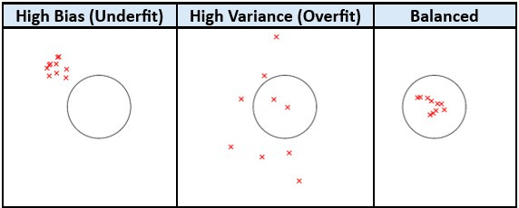
Imagine, you are trying to hit the target with arrows.
In underfitting (high bias), attempted arrows are mostly consistent but away from the target — showing that the model needs some more info to capture the pattern.
In overfitting (high variance), arrows are scattered all over including the target. The model captures the pattern, but the performance is not stable.
A balanced model generalizes well and is optimal level of bias and variance.
How to Keep ML Models Under Check?
It’s Regularization.
Regularization helps to keep your ML model on track by shrinking, removing, or simplifying model parameters (weights). The objective of regularization is to make model simpler – but not the simplest. Simpler models with regularization often make better predictions.
Now we’ll discuss how techniques like L0, L1, and L2 regularization improve generalization, reduce errors, and lead to more efficient models.
What is Regularization?
Regularization is a way to keep your model from getting too complicated.
Think of it as telling your model, “Don’t overthink it.”
It works by adding a penalty to the loss function, which discourages the model from getting too complex.
Base Loss Function: MSE
Let’s start with the standard Mean Squared Error (MSE) loss:
We minimize this to train models. But if we add regularization, we modify the loss function as below:
Loss = MSE + 𝜆 Penalty … … (1)
Here, 𝜆 controls how much penalty to apply. And the penalty depends on the type of regularization.
The Three Types of Regularization
There are Three regularization techniques L0, L1, and L2. Let’s understand them in simple terms.
L0 Regularization – ‘Pick the Fewest’
This is the ideal regularization technique that wants to add the minimum number of features to use in a model and hence, adds penalty to the number of non-zero weights.
The term ||w||o defines the number of non-zero weights in a weight vector. For example,
then
So, L0 regularization pushes the model to use as few features as possible. It’s like packing for a trip with strict baggage limits—you only bring what’s absolutely essential. And hence, most weights drop to exactly zero and results in a minimal, highly sparse model.
L1 Regularization (Lasso) – ‘Drop Some’
Here the penalty factor is the sum of absolute weights:
So, L1 regularization pushes some weights drop to zero. It’s like you’ve got limited luggage space, so you pack only what you’ll actually use. With this, it automatically selects the most important features that truly matter. Hence helps in feature selection also.
L2 Regularization (Ridge) – ‘Shrink All’
Here the penalty factor is the sum of squared weights:
L2 regularization shrinks all weights without setting them to zero. It’s like, you can pack everything, but it all has to fit in a carry-on. This is used when every feature adds value, but none should dominate.
How is the Penalty Function Optimized during Training?
L0 regularization decides which features should stay and which should go. It’s a combinatorial optimization problem. Since it’s not differentiable or convex, standard optimization methods like gradient descent won’t work. Instead, it relies on greedy algorithms, heuristics, or brute force — similar to traditional feature selection.
So, though L0 provides the best regularization model, it is computationally expensive, hardest to optimize, and difficult to execute.
Hence, we mostly use L1 and L2.
L1 regularization is convex but not smooth, making it moderately easy to optimize with specialized methods; it promotes sparsity by setting some weights to zero.
L2 regularization is both convex and smooth, making it the easiest to optimize using standard methods, and it shrinks weights without eliminating them.
A simple summary is provided below:
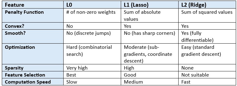
SUMMARY
Regularization helps ML models stay simple, avoid overfitting, and generalize better.
By shrinking, dropping, or limiting weights using L0, L1, or L2 methods, we find the right balance between bias and variance.
In ML, simpler models often perform better and that’s the power of ‘less is more’.
Simplicity is a strategy. Keep it simple. Make it smart.