
Why We Need Matrices & GPUs for Deep Learning
A simple illustration of how matrices and GPUs work together...

Deep learning rs on massive neural networks with billions of parameters, especially in fields like computer vision, NLP, and LLMs. This raises a key question: how are such large computations handled efficiently?
In this article, we’ll use simple examples to show how matrices and GPUs make it possible — leveraging matrix properties like additivity and associativity.
So, we already know that deep learning consists of massive neural networks built with varying architectures. With the rise of ground-breaking applications in computer vision, natural language processing (NLP), and large language models (LLMs), the scale of such neural networks has become unimaginable and often to the tune of billion parameters.
This raises an important question: How exactly do we handle such massive computations efficiently?
In this article, we will take an insider look at how exactly matrices and GPUs (Graphics Processing Units) help handling such large-scale deep learning models.
Please note that, for illustration, a massive real-life neural network will be difficult to imagine. Hence, we will use only a very simple neural network just to drive the concept. So, let’s understand the mechanism.
ILLUSTRATION
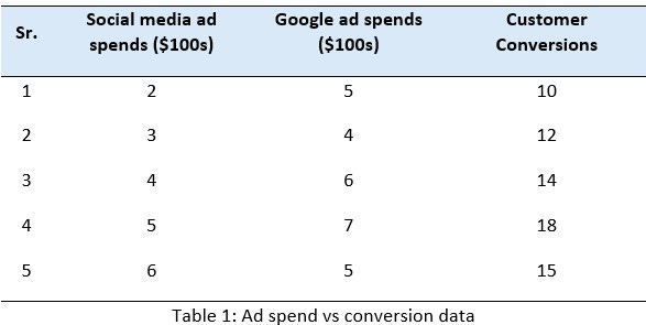
Let us consider the data below that captures how Social-Media and Google ad-spend influence customer conversions. We want to train a neural network on it.
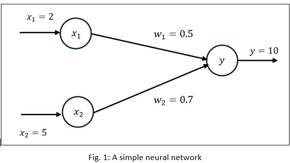
Let us consider the world’s simplest Neural Network and see how it is trained on the above data. To keep it even simpler, we ignore any hidden layer, activation function, and bias. However, the concept works for all large scale complex neural models.
Since there are two inputs (ad-spends) and one output (conversions), we consider two input neurons.
Consider two weight factors as below - i.e. inputs with random initial values w1 = 0.5 and w2 = 0.7:
Assume learning rate i.e., a small step size for updates:

Now, let’s take the first row of the data as inputs x1 = 2 and x2 = 5 and the target output y = 10.
We will do the calculations for forward pass and backpropagation to adjust weights for the first row of the training data set.
We will do the calculations first in simple manual steps:
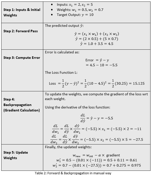
I must say, this is a highly trivial process and does not scale up for more complex settings! Now, let us see how we can put a structure around it for scalability and easy handling. Ideally the matrices way!
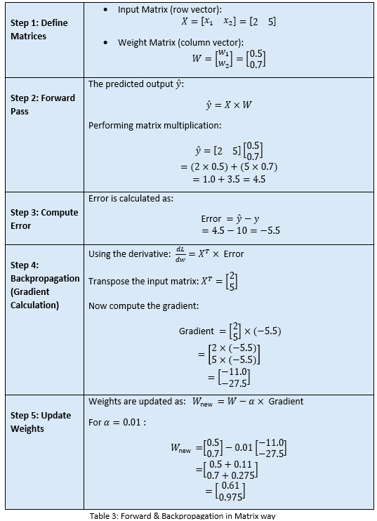
We got the same results with matrices. But in a more clean and structured way.
WEIGHT OPTIMIZATION STRATEGY: BATCH SELECTION
We have used the first row only to optimize the random weights. Now, continue the process for all 5 rows in the dataset. After going through all rows (one full pass through the dataset), we complete one epoch. We repeat multiple epochs until the weights converge to optimal values.
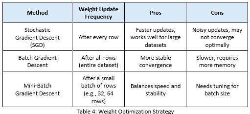
For the full training dataset, we have three possible weight optimization strategies:
Stochastic Gradient Descent (SGD): Updates weights after each row (what we did so far). The term ‘stochastic’ comes from probability and randomness. In Stochastic Gradient Descent (SGD), the gradient is computed using only one random sample at a time, instead of the entire dataset.
Batch Gradient Descent: Updates weights after all rows in one go. Unlike Stochastic Gradient Descent (SGD) which updates weights after each row, Batch Gradient Descent updates weights only once per full dataset.
Mini-Batch Gradient Descent: Uses a small batch of rows before updating weights. Mini-Batch Gradient Descent updates weights after processing a small batch of rows (e.g., 32, 64 rows at a time).
Key Differences Between SGD and Batch Gradient Descent
Which One to Use – A Thumb Rule
SGD: If you have a huge dataset and need faster updates.
Mini-Batch: If you want a balance between efficiency and stability (used in most deep learning models).
Batch Gradient Descent: If you have a small dataset and can afford full-batch training.
Whatever the weight optimization strategy is, we see that using matrix operations, especially multiplication, it makes neural networks efficient, scalable, and simple. With many neurons, computing each one separately is slow. Matrices let us calculate multiple neurons at once during forward and backward passes.
How GPUs Leverage Matrices to Accelerate Deep Learning
Now that we understand how matrices help in managing a large-scale neural network in deep learning models, let us see how GPUs take advantage of matrices properties to optimize hardware and parallel computation.
At the core, it is matrix multiplication for forward and backpropagation. If matrix multiplications can be done in parallel, that will help turbocharge neural networks and deep learning models.
GPUs can perform these multiplications in parallel, which makes training very fast. Matrix notation allows quick, vectorized calculations and helps scale to large neural networks. It also speeds up backpropagation and works efficiently with tools like TensorFlow and PyTorch.
Now, let’s understand how GPUs help speed up matrix multiplication, which lies at the core of neural networks with a simple example. Again the concept goes for more complex matrices.
Let's take two simple matrices, A and B:
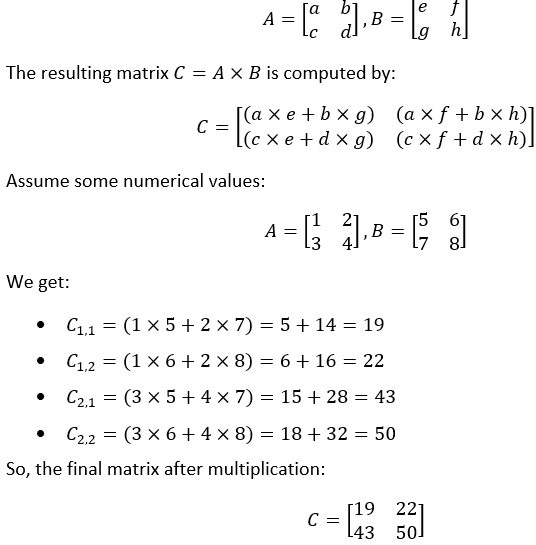
MATRIX MULTIPLICATION WITH GPU
A GPU typically assigns each element of the resulting matrix to a separate core (or thread) or parallel computation. For the above 2 X 2 matrix multiplication, we have 4 elements, and thus 4 parallel tasks. Each element calculation becomes its own small job:
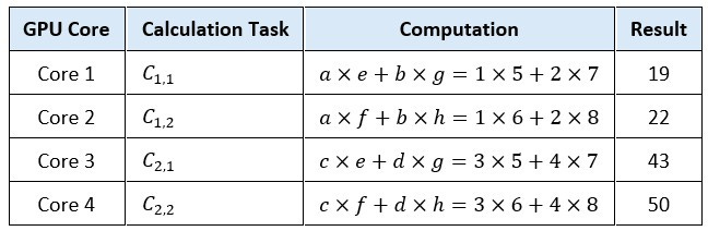
Each GPU core independently calculates one element simultaneously. This greatly reduces total computation time for large matrices.
MATRIX SPLITTING & JOINING IN GPUS
In several other situations, the size of the matrices are huge and can be millions of rows/columns. In such cases, each matrix may be decomposed into smaller sizes, processed, and added back for the full output.
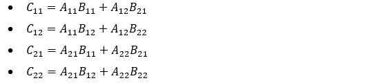
Here is an example of multiplication of two 4 X 4 matrices where the matrices are split, multiplied block-wise in parallel, and recombined:
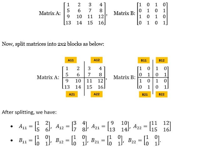
Each block can be assigned to different cores, and the multiplication can be computed independently. And that is how GPUs can help with parallel processing.
Here's the step-by-step calculation for C11:
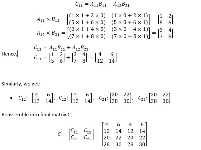
So, we see that subsets of a matrix can be computed independently by different GPU cores and then recombined. Matrix properties like associativity and additivity make this parallel computation possible and efficient in GPUs.
SUMMARY
Deep learning relies on large neural networks with many layers and neurons to learn complex patterns from data. These networks are trained using forward and backward propagation, where matrix multiplication is used to compute errors and update weights accordingly during the training process.
Since these operations involve large amounts of data, GPUs accelerate the process by performing matrix multiplications in parallel, leveraging the additive and associative properties of matrices to compute multiple values at once in different cores — making training faster and more efficient.
Hope this article helps to understand the fundamentals.